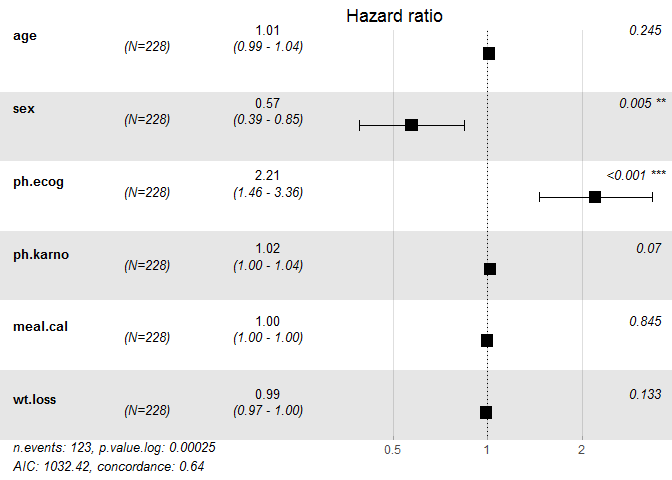
Forest plot for cox model
建立cox模型
library(survival)  #载入包
cox_model <- coxph(Surv(time, status) ~ age + sex + ph.ecog + ph.karno + meal.cal + wt.loss, data = lung)  #建立cox回归模型
summary(cox_model)
## Call:
## coxph(formula = Surv(time, status) ~ age + sex + ph.ecog + ph.karno +
##     meal.cal + wt.loss, data = lung)
##
##   n= 170, number of events= 123
##    (58 observations deleted due to missingness)
##
##                coef  exp(coef)   se(coef)      z Pr(>|z|)
## age       1.346e-02  1.014e+00  1.157e-02  1.163 0.244805
## sex      -5.570e-01  5.729e-01  1.986e-01 -2.805 0.005039 **
## ph.ecog   7.943e-01  2.213e+00  2.129e-01  3.731 0.000191 ***
## ph.karno  1.985e-02  1.020e+00  1.097e-02  1.809 0.070381 .
## meal.cal -5.028e-05  9.999e-01  2.570e-04 -0.196 0.844890
## wt.loss  -1.136e-02  9.887e-01  7.573e-03 -1.501 0.133439
## ---
## Signif. codes:  0 '***' 0.001 '**' 0.01 '*' 0.05 '.' 0.1 ' ' 1
##
##          exp(coef) exp(-coef) lower .95 upper .95
## age         1.0135     0.9866    0.9908    1.0368
## sex         0.5729     1.7454    0.3882    0.8456
## ph.ecog     2.2129     0.4519    1.4580    3.3588
## ph.karno    1.0201     0.9803    0.9983    1.0422
## meal.cal    0.9999     1.0001    0.9994    1.0005
## wt.loss     0.9887     1.0114    0.9741    1.0035
##
## Concordance= 0.636  (se = 0.03 )
## Rsquare= 0.141   (max possible= 0.998 )
## Likelihood ratio test= 25.78  on 6 df,   p=0.0002452
## Wald test            = 24.93  on 6 df,   p=0.0003516
## Score (logrank) test = 25.43  on 6 df,   p=0.0002846
C-index and CI
The C-statistic(“concordance” statistic or C-index) is a measure of goodness of fit for binary outcomes in a logistic regression model. In clinical studies, the C-statistic gives the probability a randomly selected patient who experienced an event (e.g. a disease or condition) had a higher risk score than a patient who had not experienced the event. It is equal to the AUC of ROC and ranges from 0.5 to 1.
c_index <- summary(cox_model)$concordance
c_index
##          C      se(C)
## 0.63598440 0.03028917
95%可信区间可通过(C-1.96se, C+1.96se)计算, 结果为95% CI (0.57661,0.69535)
library(survminer)
ggforest(cox_model, main = "Hazard ratio",cpositions = c(0.02, 0.22, 0.4), fontsize = 0.8,refLabel = "reference", noDigits = 2)
#cpositions设置图中前三列的相对位置
#fontsize为字体大小
#refLabel 设定参考组标签
#noDigits显示数字位数
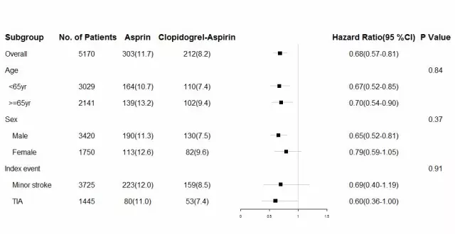
Forestplot method
用R包forestplot解决该问题。首先我们需要整理数据为想要显示的格式。
#install.packages("forestplot")
library(forestplot)
dat <- read.csv2("https://raw.githubusercontent.com/chenyuan-date/Data/master/Forest-plot-data.csv", sep = ",", header = T, stringsAsFactors = F, na.strings = "NA")
dat
##            Subgroup No..of.Patients    Asprin Clopidogrel.Aspirin
## 1           Overall            5170 303(11.7)            212(8.2)
## 2               Age              NA
## 3             <65yr            3029 164(10.7)            110(7.4)
## 4            >=65yr            2141 139(13.2)            102(9.4)
## 5               Sex              NA
## 6              Male            3420 190(11.3)            130(7.5)
## 7            Female            1750 113(12.6)             82(9.6)
## 8       Index event              NA
## 9      Minor stroke            3725 223(12.0)            159(8.5)
## 10              TIA            1445  80(11.0)             53(7.4)
##    Hazard.Ratio.95..CI. P.Value    X  X.1  X.2
## 1       0.68(0.57-0.81)         0.68 0.57 0.81
## 2                          0.84
## 3       0.67(0.52-0.85)         0.67 0.52 0.85
## 4       0.70(0.54-0.90)          0.7 0.54  0.9
## 5                          0.37
## 6       0.65(0.52-0.81)         0.65 0.52 0.81
## 7       0.79(0.59-1.05)         0.79 0.59 1.05
## 8                          0.91
## 9       0.69(0.40-1.19)         0.69  0.4 1.19
## 10      0.60(0.36-1.00)          0.6 0.36    1
forestplot(as.matrix(dat[,1:6]), dat[7:9], graph.pos=5, graphwidth = unit(50,"mm"), is.summary = c(TRUE,rep(FALSE,10)), boxsize=0.2, line.margin=unit(1,"mm"), lineheight = unit(10,'mm'), colgap = unit(3,"mm"), zero=1, xticks = c(0.0,0.5,1.0,1.5))

#要用数据的前6列作为文本,数据要转换为矩阵形式,故用as.matrix函数。
#紧随的三项是均值和95%CI的上下限,用来绘制森林图的效应值及其误差线。
#输入vignette("forestplot", package="forestplot")查看更详细用法