Univariate and Multivariate Survival Analysis
Introduction
Techniques of survival analysis are needed once you have right-censored data. Such data is the result of clinical trials or retrospective studies that observe a defined endpoint such as progression free survival (PFS) or overall survival (OS).
Data source
The survivalAnalysis package assumes the data is a data frame with one row per subject and at least two columns: - A numeric column giving the survival time. - A logical or numeric (0/1) column with the censoring indicator. TRUE or 1 is interpreted such that the endpoint occurred for the subject at the given time, FALSE or 0 is interpreted such that the endpoint did not occur during the given time under observation.
suppressPackageStartupMessages(library(survival))
head(lung) #Survival data is contained in the "time" and "status" columns, with all other columns as presumed or potential covariates.
##   inst time status age sex ph.ecog ph.karno pat.karno meal.cal wt.loss
## 1    3  306      2  74   1       1       90       100     1175      NA
## 2    3  455      2  68   1       0       90        90     1225      15
## 3    3 1010      1  56   1       0       90        90       NA      15
## 4    5  210      2  57   1       1       90        60     1150      11
## 5    1  883      2  60   1       0      100        90       NA       0
## 6   12 1022      1  74   1       1       50        80      513       0
The Analysis Result
suppressPackageStartupMessages(library(tidyverse))
suppressPackageStartupMessages(library(tidytidbits))
## Warning: package 'tidytidbits' was built under R version 3.5.2
library(survivalAnalysis)
#perform an analysis generating a result object, and then perform output such as printing or plotting using this object.
## Warning: package 'survivalAnalysis' was built under R version 3.5.2
# Overview of data and check the median survival
survival::lung %>%
  analyse_survival(vars(time, status))
# vars() is from dplyr, allows to give the plain variable names. Passing column names as strings is also possible.
## Overall Analysis:
##          log.rank.p   n median Lower.CI Upper.CI min    max
## overall:       <NA> 228  310.0    285.0    363.0 5.0 1022.0
##
## <only one group in analysis>
survival::lung %>%
  analyse_survival(vars(time, status)) %>%
  print(timespan_unit="months")
## Overall Analysis:
##          log.rank.p   n median Lower.CI Upper.CI min  max
## overall:       <NA> 228   10.2      9.3     11.9 0.2 33.5
##
## <only one group in analysis>
Univariate Survival Analysis
survival::lung %>% #The ECOG performance status is a classical prognostic indicator.
  count_by(ph.ecog) #count_by method from tidytidbits to check the distribution of "ph.ecog"
## # A tibble: 5 x 4
##   ph.ecog     n     rel percent
##     <dbl> <int>   <dbl> <chr>
## 1       0    63 0.276   27.6%
## 2       1   113 0.496   49.6%
## 3       2    50 0.219   21.9%
## 4       3     1 0.00439 " 0.4%"
## 5      NA     1 0.00439 " 0.4%"
survival analysis comparing the subgroups formed by the ECOG status
survival::lung %>%
  mutate(ecog=recode_factor(ph.ecog, `0`="0", `1`="1", `2`="2-3", `3`="2-3")) %>% #group 2 und 3 together
  analyse_survival(vars(time, status), by=ecog) -> result #store the result object for later use
print(result)
## Analysis by ecog:
## Overall Analysis:
##          log.rank.p   n median Lower.CI Upper.CI min    max
## overall:    p<0.001 227  310.0    285.0    363.0 5.0 1022.0
##
## Descriptive Statistics per Subgroup:
##     records events median Lower.CI Upper.CI
## 0        63     37  394.0    348.0    574.0
## 1       113     82  306.0    268.0    429.0
## 2-3      51     45  183.0    153.0    288.0
##
## Pair-wise p-values (log-rank, uncorrected):
##         0     1
## 1   0.063    NA
## 2-3   0.0 0.003
##
## Pair-wise Hazard Ratios:
##           Lower.CI   HR Upper.CI      p
## 1 vs. 0       0.98 1.45     2.13  0.064
## 0 vs. 1       0.47 0.69     1.02  0.064
## 2-3 vs. 0     1.64 2.54     3.93 <0.001
## 0 vs. 2-3     0.25 0.39     0.61 <0.001
Instead of inserting a mutate call, we just pass the logical expression ph.ecog <= 1
survival::lung %>%
  analyse_survival(vars(time, status),
                   by=ph.ecog <= 1,
                   by_label_map=c(`TRUE`="ECOG 0-1", #give labels to the values of `by`. These labels will also be used in plots
                                  `FALSE`="ECOG 2-3"))
## Analysis by ph.ecog <= 1:
## Overall Analysis:
##          log.rank.p   n median Lower.CI Upper.CI min    max
## overall:    p<0.001 227  310.0    285.0    363.0 5.0 1022.0
##
## Descriptive Statistics per Subgroup:
##          records events median Lower.CI Upper.CI
## ECOG 0-1     176    119  353.0    306.0    433.0
## ECOG 2-3      51     45  183.0    153.0    288.0
##
## Hazard Ratio:
##                       Lower.CI  HR Upper.CI      p
## ECOG 2-3 vs. ECOG 0-1     1.41 2.0     2.82 <0.001
## ECOG 0-1 vs. ECOG 2-3     0.35 0.5     0.71 <0.001
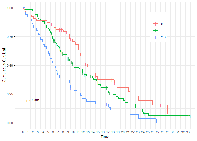
Kaplan-Meier Plots
The survminer package has revolutionized drawing of Kaplan-Meier plots in R. The survivalAnalysis package fully integrates plotting with survminer, providing sane defaults:
kaplan_meier_plot(result)
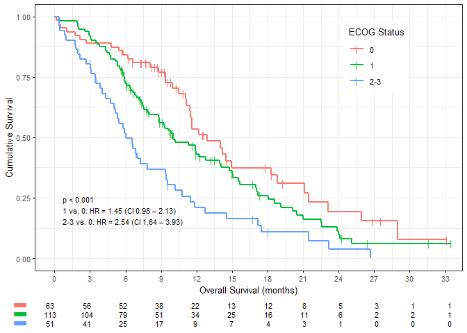
Refine parameters, refer to the parameters in function ggsurvplot. All parameters supported by ggsurvplot can simply be passed to kaplan_meier_plot. In addition, there are some shortcuts which we will now use.
kaplan_meier_plot(result,
                  break.time.by="breakByQuarterYear", #x axis breaks by quarter year
                  xlab=".OS.months", #x axis label for OS
                  legend.title="ECOG Status", #legend label
                  hazard.ratio=T, #display the hazard ratios
                  risk.table=TRUE, #display risk table
                  table.layout="clean", #risk table "clean" only with minimal overhead
                  ggtheme=ggplot2::theme_bw(10)) #custom theme
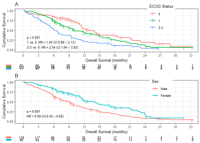
Two KM plots side-by-side using kaplan_meier_grid. This piece of code also demonstrates the possible use of lists of default arguments, which can be overridden. If arguments differ per-plot, there is the mapped_plot_args argument.
Internally, gridExtra::marrangeGrob does the layout. For some reason, the returned value needs an explicit print. Normally you will want to save it to PDF. I recommend using tidytidbits’ save_pdf, into which you can simply pipe the kaplan_meier_grid output.
default_args <- list(break.time.by="breakByMonth",
                     xlab=".OS.months",
                     legend.title="ECOG Status",
                     hazard.ratio=T,
                     risk.table=TRUE,
                     table.layout="clean",
                     ggtheme=ggplot2::theme_bw(10))

list(result,
     survival::lung %>%
       analyse_survival(vars(time, status),
                        by=sex,
                        by_label_map=c(`1`="Male", `2`="Female"))
     ) %>%
  kaplan_meier_grid(nrow=2,
                    default_args,
                    break.time.by="breakByQuarterYear",
                    mapped_plot_args=list(
                      legend.title=c("ECOG Status", "Sex"),
                      title=c("A", "B")
                    )) %>%
  print
Multivariate Survival Analysis
Multivariate analysis, using the technique of Cox regression, is applied when there are multiple, potentially interacting covariates. While the log-rank test and Kaplan-Meier plots require categorical variables, Cox regression works with continuous variables. (Of course, you can use it with categorical variables as well, but this has implications which are described below.)
In lung data, possibly interesting covariates are patient age, sex, ECOG status and the amount of weight loss. Sex is encoded as a numerical vector, but is in fact categorical. We need to make it a factor. ECOG status is at least ordinally scaled, so we leave it numerical for now. Following the two-step philosophy of survivalAnalysis, we first perform the analysis with analyse_multivariate and store the result object. We provide readable labels for the covariates to allow easy interpretation. There is a print() implementation which prints essential information for our result.
covariate_names <- c(age="Age at Dx", #provide readable labels for the covariates to allow easy interpretation.
                     sex="Sex",
                     ph.ecog="ECOG Status",
                     wt.loss="Weight Loss (6 mo.)",
                     `sex:female`="Female",
                     `ph.ecog:0`="ECOG 0",
                     `ph.ecog:1`="ECOG 1",
                     `ph.ecog:2`="ECOG 2",
                     `ph.ecog:3`="ECOG 3")

survival::lung %>%
  mutate(sex=rename_factor(sex, `1` = "male", `2` = "female")) %>% #make sex a factor.
  analyse_multivariate(vars(time, status),
                       covariates = vars(age, sex, ph.ecog, wt.loss),
                       covariate_name_dict = covariate_names) -> result #store the result object.
print(result)
## Overall:
##    n                 covariates Likelihood ratio test p Wald test p
##  213 age, sex, ph.ecog, wt.loss                  <0.001      <0.001
##  Score (logrank) test p
##                  <0.001
##
## Hazard Ratios:
##   factor.id         factor.name factor.value   HR Lower_CI Upper_CI Inv_HR
##  sex:female                 Sex       female 0.55     0.39     0.78   1.81
##     wt.loss Weight Loss (6 mo.) <continuous> 0.99     0.98      1.0   1.01
##         age           Age at Dx <continuous> 1.01     0.99     1.03   0.99
##     ph.ecog         ECOG Status <continuous> 1.67     1.31     2.14    0.6
##  Inv_Lower_CI Inv_Upper_CI      p
##          1.28         2.55 <0.001
##           1.0         1.02  0.176
##          0.97         1.01  0.165
##          0.47         0.76 <0.001
A Note on Categorical Variables
Inv_HR: for binary variables, it means inverted HR, equal to 1/HR.
Things get more complicated with three or more categories. The rule is: You must choose one level of the factor as the reference level with defined hazard ratio 1.0. Then, for k levels, there will be k-1 pseudo variables created which represent the hazard ratio of this level compared to subjects in the reference level. (For the comparison of one level vs. all remaining subjects see the paragraph on one-hot analysis further down.)
As an example, we consider the two covariates which were significant above, sex and ECOG, and regard the ECOG status as a categorical variable with four levels. As reference level, we choose ECOG=0 with the parameter reference_level_dict.
survival::lung %>%
  mutate(sex=rename_factor(sex, `1` = "male", `2` = "female"),
         ph.ecog = as.factor(ph.ecog)) %>%
  analyse_multivariate(vars(time, status),
                       covariates = vars(sex, ph.ecog),
                       covariate_name_dict=covariate_names,
                       reference_level_dict=c(ph.ecog="0"))
## Overall:
##    n   covariates Likelihood ratio test p Wald test p
##  227 sex, ph.ecog                  <0.001      <0.001
##  Score (logrank) test p
##                  <0.001
##
## Hazard Ratios:
##   factor.id factor.name factor.value   HR Lower_CI Upper_CI Inv_HR
##  sex:female         Sex       female 0.58     0.42     0.81   1.72
##   ph.ecog:1 ECOG Status            1 1.52     1.03     2.25   0.66
##   ph.ecog:2 ECOG Status            2 2.58     1.66     4.01   0.39
##   ph.ecog:3 ECOG Status            3 7.76     1.04    58.04   0.13
##  Inv_Lower_CI Inv_Upper_CI      p
##          1.24          2.4  0.001
##          0.45         0.97  0.036
##          0.25          0.6 <0.001
##          0.02         0.96  0.046
A Forest Plot
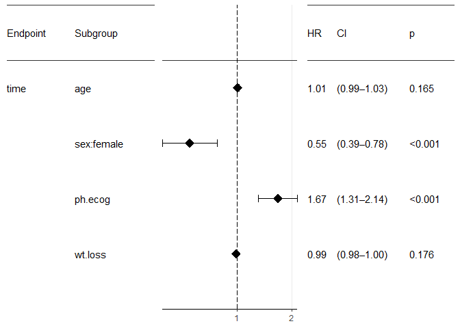
The usual method to display results of multivariate analyses is the forest plot. The survivalAnalysis package provides an implementation which generates ready-to-publish plots and allows extensive customization.
forest_plot(result)
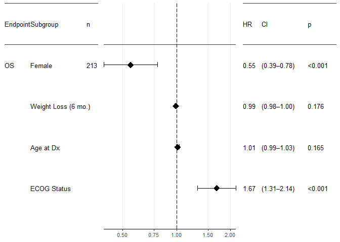
Tune parameters
forest_plot(result,
            factor_labeller = covariate_names, #label the subgroups.
            endpoint_labeller = c(time="OS"), #label the endpoint.
            orderer = ~order(HR), #order by hazard ratio
            labels_displayed = c("endpoint", "factor", "n"),
            ggtheme = ggplot2::theme_bw(base_size = 10), #Adjust font size
            relative_widths = c(1, 1.5, 1), #more space for the plot, less space for the tables
            HR_x_breaks = c(0.25, 0.5, 0.75, 1, 1.5, 2)) #more breaks on the X axis
The forest_plot function actually accepts any number of results and will display them all in the same plot. For example, you may want to display both OS and PFS in the same plot, but of course ordered and with a line separating the two. To do that,
- throw both results into
forest_plot - order first by endpoint, then by something else: orderer = ~order(endpoint, factor.name)
- use a categorizer function returning a logical vector which determines where the separating line shall be drawn. For a flexible solution, the usual idiom is something like categorizer = ~!sequential_duplicates(endpoint, ordering = order(endpoint, factor.name)), where the ordering clause is identical to your orderer code.
Finally, if you want separate plots but display them in a grid, useforest_plot_gridto do the grid layout and forest_plot’s title argument to add the A, B, C. labels.
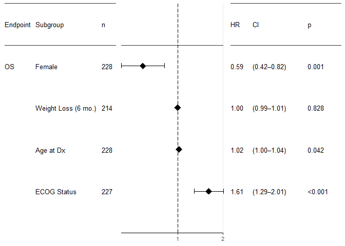
Multiple Univariate Analyses
It is common practice to perform univariate analyses of all covariates first and take only those into the multivariate analysis which were significant to some level in the univariate analysis. (I see some pros and strong cons with this procedure, but am open to learn more on this). The univariate part can easily be achieved using purrr’s map function. A forest plot will plot multiple results, even if they come as a list.
df <- survival::lung %>% mutate(sex=rename_factor(sex, `1` = "male", `2` = "female"))

map(vars(age, sex, ph.ecog, wt.loss), function(by)
{
  analyse_multivariate(df,
                       vars(time, status),
                       covariates = list(by), # covariates expects a list
                       covariate_name_dict = covariate_names)
}) %>%
  forest_plot(factor_labeller = covariate_names,
              endpoint_labeller = c(time="OS"),
              orderer = ~order(HR),
              labels_displayed = c("endpoint", "factor", "n"),
              ggtheme = ggplot2::theme_bw(base_size = 10))
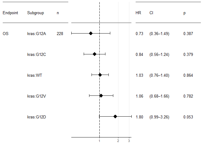
One-Hot Encoding
The one-hot parameter triggers a mode where for each factor level, the hazard ratio vs. the remaining cohort is plotted. This means that no level is omitted. Please be aware of the statistical caveats. And please note that this has nothing to do any more with multivariate analysis. In fact, now you need the result of the univariate, categorically-minded analyse_survival.
survival::lung %>%
  mutate(kras=sample(c("WT", "G12C", "G12V", "G12D", "G12A"),
                     nrow(.),
                     replace = T,
                     prob = c(0.6, 0.24, 0.16, 0.06, 0.04))
          ) %>%
  analyse_survival(vars(time, status), by=kras) %>%
  forest_plot(use_one_hot=TRUE,
              endpoint_labeller = c(time="OS"),
              orderer = ~order(HR),
              labels_displayed = c("endpoint", "factor", "n"),
              ggtheme = ggplot2::theme_bw(base_size = 10))