Compare and select machine learning models
When you have a new dataset it is a good idea to visualize the data using a number of different graphing techniques in order to look at the data from different perspectives.
The same idea applies to model selection. You should use a number of different ways of looking at the estimated accuracy of your machine learning algorithms in order to choose the one or two to finalize.
The way that you can do that is to use different visualization methods to show the average accuracy, variance and other properties of the distribution of model accuracies.
data preparation
# load libraries
library(mlbench) #include diabetes data
library(caret)

# load the dataset
data(PimaIndiansDiabetes)
head(PimaIndiansDiabetes)
##   pregnant glucose pressure triceps insulin mass pedigree age diabetes
## 1        6     148       72      35       0 33.6    0.627  50      pos
## 2        1      85       66      29       0 26.6    0.351  31      neg
## 3        8     183       64       0       0 23.3    0.672  32      pos
## 4        1      89       66      23      94 28.1    0.167  21      neg
## 5        0     137       40      35     168 43.1    2.288  33      pos
## 6        5     116       74       0       0 25.6    0.201  30      neg
Train Models
# prepare training scheme
control <- trainControl(method="repeatedcv", number=10, repeats=3)
# CART: Classification and Regression Trees
set.seed(7)
library(rpart)
fit.cart <- train(diabetes~., data=PimaIndiansDiabetes, method="rpart", trControl=control)
# LDA: Linear Discriminant Analysis
set.seed(7)
fit.lda <- train(diabetes~., data=PimaIndiansDiabetes, method="lda", trControl=control)
# SVM: Support Vector Machine with Radial Basis Function
set.seed(7)
fit.svm <- train(diabetes~., data=PimaIndiansDiabetes, method="svmRadial", trControl=control)
# kNN: k-Nearest Neighbors
set.seed(7)
fit.knn <- train(diabetes~., data=PimaIndiansDiabetes, method="knn", trControl=control)
# Random Forest
set.seed(7)
fit.rf <- train(diabetes~., data=PimaIndiansDiabetes, method="rf", trControl=control)
# glmnet (lasso/ridge/elastic net)
set.seed(7)
fit.glmnet <- train(diabetes~., data=PimaIndiansDiabetes, method="glmnet", trControl=control)
# collect resamples
results <- resamples(list(CART=fit.cart, LDA=fit.lda, SVM=fit.svm, KNN=fit.knn, RF=fit.rf, GLMNET=fit.glmnet))
We trainned the 5 machine learning models that we will compare in the next section.
We use repeated cross validation with 10 folds and 3 repeats, a common standard configuration for comparing models. The evaluation metric is accuracy and kappa because they are easy to interpret.
After the models are trained, they are added to a list and resamples() is called on the list of models. This function checks that the models are comparable and that they used the same training scheme (trainControl configuration). This object contains the evaluation metrics for each fold and each repeat for each algorithm to be evaluated.
Compare Models
8 different techniques for comparing the estimated accuracy of the constructed models
Table Summary
Create a table with one algorithm for each row and evaluation metrics for each column. In this case we have sorted.
# summarize differences between modes
summary(results)
##
## Call:
## summary.resamples(object = results)
##
## Models: CART, LDA, SVM, KNN, RF, GLMNET
## Number of resamples: 30
##
## Accuracy
##             Min.   1st Qu.    Median      Mean   3rd Qu.      Max. NA's
## CART   0.6233766 0.7114662 0.7402597 0.7381864 0.7759740 0.8441558    0
## LDA    0.6710526 0.7532468 0.7662338 0.7759455 0.8051948 0.8701299    0
## SVM    0.6710526 0.7402597 0.7582023 0.7650946 0.7889610 0.8961039    0
## KNN    0.6184211 0.6983510 0.7320574 0.7299385 0.7532468 0.8181818    0
## RF     0.6842105 0.7296651 0.7582023 0.7625370 0.7922078 0.8571429    0
## GLMNET 0.6842105 0.7557245 0.7662338 0.7772613 0.8019481 0.8701299    0
##
## Kappa
##             Min.   1st Qu.    Median      Mean   3rd Qu.      Max. NA's
## CART   0.1584699 0.3295590 0.3765182 0.3934073 0.4684788 0.6393443    0
## LDA    0.2484177 0.4195842 0.4515939 0.4800991 0.5511677 0.7047546    0
## SVM    0.2187500 0.3888801 0.4167479 0.4520197 0.5002572 0.7638037    0
## KNN    0.1112903 0.3228267 0.3866876 0.3818558 0.4382002 0.5866564    0
## RF     0.2852665 0.3860329 0.4552584 0.4613026 0.5168514 0.6780692    0
## GLMNET 0.2715655 0.4388664 0.4562546 0.4831300 0.5427711 0.6994536    0
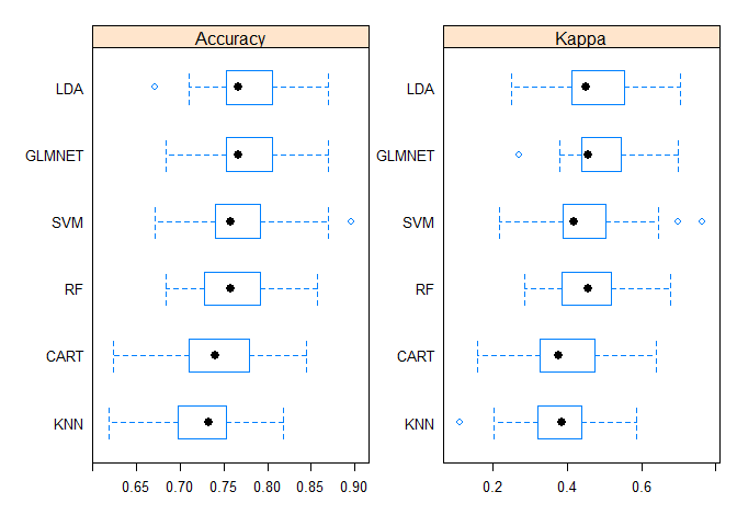
Box and Whisker Plots
The boxes are ordered from highest to lowest mean accuracy.
# box and whisker plots to compare models
scales <- list(x=list(relation="free"), y=list(relation="free"))
bwplot(results, scales=scales)
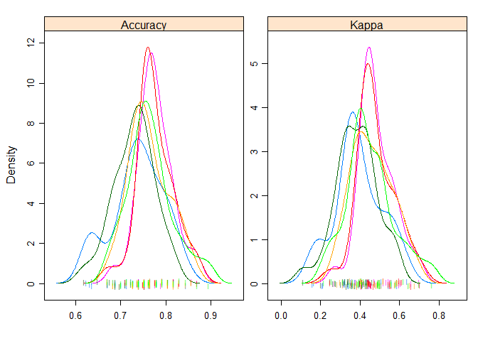
Density Plots
A useful way to evaluate the overlap in the estimated behavior of algorithms.
# density plots of accuracy
scales <- list(x=list(relation="free"), y=list(relation="free"))
densityplot(results, scales=scales, pch = "|")
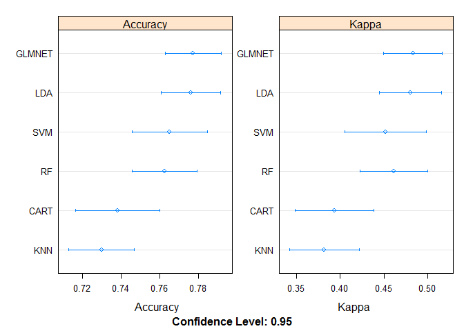
Dot Plots
# dot plots of accuracy
scales <- list(x=list(relation="free"), y=list(relation="free"))
dotplot(results, scales=scales)
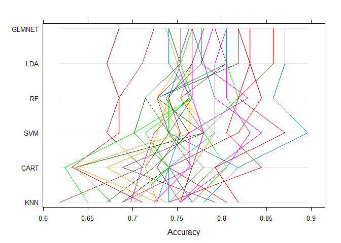
Parallel Plots
It shows how each trial of each cross validation fold behaved for each of the algorithms tested. It can help you see how those hold-out subsets that were difficult for one algorithms faired for other algorithms.
# parallel plots to compare models
parallelplot(results)
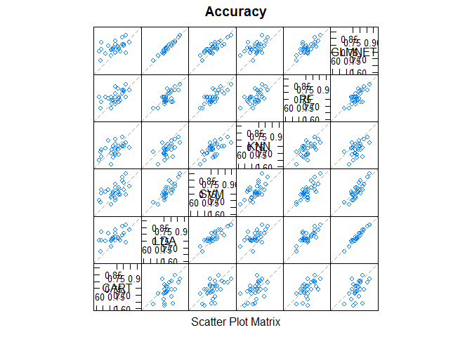
Scatterplot Matrix
This is invaluable when considering whether the predictions from two different algorithms are correlated. If weakly correlated, they are good candidates for being combined in an ensemble prediction.
# pair-wise scatterplots of predictions to compare models
splom(results)
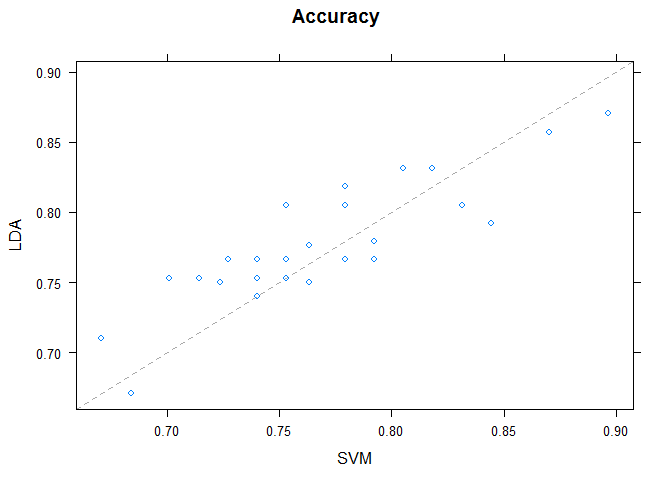
Pairwise xyPlots
One can zoom in on one pair-wise comparison of the accuracy of trial-folds for two machine learning algorithms with an xyplot.
# xyplot plots to compare models
xyplot(results, models=c("LDA", "SVM"))
Statistical Significance Tests
You can calculate the significance of the differences between the metric distributions of different machine learning algorithms. We can summarize the results directly by calling the summary() function.
# difference in model predictions
diffs <- diff(results)
# summarize p-values for pair-wise comparisons
summary(diffs)
##
## Call:
## summary.diff.resamples(object = diffs)
##
## p-value adjustment: bonferroni
## Upper diagonal: estimates of the difference
## Lower diagonal: p-value for H0: difference = 0
##
## Accuracy
##        CART     LDA       SVM       KNN       RF        GLMNET
## CART            -0.037759 -0.026908  0.008248 -0.024351 -0.039075
## LDA    0.007510            0.010851  0.046007  0.013409 -0.001316
## SVM    0.137937 0.508550             0.035156  0.002558 -0.012167
## KNN    1.000000 1.827e-05 0.001064            -0.032599 -0.047323
## RF     0.146186 0.362455  1.000000  0.002410            -0.014724
## GLMNET 0.005258 1.000000  0.331546  2.305e-05 0.205104
##
## Kappa
##        CART     LDA       SVM       KNN       RF        GLMNET
## CART            -0.086692 -0.058612  0.011552 -0.067895 -0.089723
## LDA    0.002322            0.028079  0.098243  0.018796 -0.003031
## SVM    0.125992 0.332610             0.070164 -0.009283 -0.031110
## KNN    1.000000 6.183e-05 0.008203            -0.079447 -0.101274
## RF     0.019422 1.000000  1.000000  0.001038            -0.021827
## GLMNET 0.001699 1.000000  0.241364  8.624e-05 1.000000